This is a Report for my Summer Open Source Project with the Stingray group (member of Open Astronomy), as a part of the Google Summer of Code 2023. Below is a detailed description and results of my project
“Quasi Periodic Oscillation detection using Gaussian Processes”
Project Abstract
In the last few Decades, we have seen a huge increase in the number of X-ray telescopes scanning the skies, allowing us to peer into distant and highly informative astronomical events. The X-ray lightcurves of many interesting events are often quasi-periodic in nature, and their origin is linked to the physics of the event making them an important tool to study these objects.
The current QPO detection methods implemented in Stingray (an Xray TimeSeries Analysis Package) are limited in scope because they are based in the frequency domains. QPO transients are heteroscedastic and non-stationary in nature, which causes a bias in the periodogram methods.
This project deals with adding a Gaussian processes feature that models the time series and performs a sampling search for model hyperparameters. GP’s are Time Domain models and mitigate many shortcomings of frequency domain methods, while also being more flexible and robust.
In this project, I have modified the code by Moritz Huebner for the the stingray library. The code makes a GPResult Class object which takes a Ligthcurve as input and performs Nested Sampling to calculate Evidences for different Models, given their Prior and Log_likelihood functions (Respective Helper functions being get_prior and get_log_likelihood).
The user essentially can make different GP Models by specifying the parameter priors, kernel types and Mean Types. The evidence can be calculated and compared to find wheather a QPO model fits the data better or a Red Noise Model, strengthening or dissmissing the case for a QPO detection. A demonstration notebook is also provided, and will be added to the Stingray Notebooks repository.
Code and Submission
The code of this project is mainly in this Pull Request: PR
The code can be understood in parallel to its usage:
1) Making a GPResult object on the lightcurve which we want to compare the Models on:
from gpmodelling import GPResult
gpresult = GPResult(Lc = lc)       # Here lc is a stingray lightcurve object
2) Creating a list of parameters of the GP model (kernel + mean function):
Any GP Model can be expressed as a kernel and a mean function, with kernel being the covariance function and mean function being the mean of the GP. We can use the already implemented Model list or create one of our own.
from gpmodelling import get_gp_params
# Implementing a Red Noise (RN kernel) and Gaussian Mean Model
get_gp_params(kernel_type= "RN", mean_type = "gaussian")
>>> ['log_arn', 'log_crn', 'log_A', 't0', 'log_sig'] # Output
3) Creating a dictionary of priors for the model parameters:
We will create a dictionary of priors for the parameters based on the lightcurve. This dictionary along with the pior list will be fed to the get_priors function which will make a Jaxns generative prior object (Used for Nested Sampling).
# Tensorflow Probability backend for the priors
import tensorflow_probability.substrates.jax as tfp
from gpmodelling import get_prior

total_time = lc.times[-1] - lc.times[0]
f = 1/(lc.times[1]- lc.times[0])
span = jnp.max(lc.counts) - jnp.min(lc.counts)
# The prior dictionary, with suitable tfpd prior distributions
prior_dict = {
    "log_A": tfpd.Uniform(low = jnp.log(0.1 * span), high= jnp.log(2 * span)),
    "t0": tfpd.Uniform(low = times[0] - 0.1*total_time, high = times[-1] + 0.1*total_time),
    "log_sig": tfpd.Uniform(low = jnp.log(0.5 * 1 / f), high = jnp.log(2 * total_time)),
    "log_arn": tfpd.Uniform(low = jnp.log(0.1 * span), high = jnp.log(2 * span)),
    "log_crn": tfpd.Uniform(low = jnp.log(1 / total_time), high = jnp.log(f)),
}
# Making a Jaxns compatible prior using the get_prior function
prior_model = get_prior(params_list2, prior_dict)
4) Creating the log_likelihood function for the model:
Here we will make a log_likelihood function which calculates the \(p(D \| \theta, M)\) , (probability of data given parameter values and Model). This will be used by the GPResult object to calculate the evidence for the model. One can also make their own log_likelihood function, given the arguments are in the same order as the parameters_list.
from gpmodelling import get_log_likelihood
likelihood_model = get_log_likelihood(params_list2, kernel_type= "RN", mean_type = "gaussian",
                                                Times = times, counts = counts)
5) Start a Nested Sampling Run on the GPResult object:
We can now run the Nested Sampler on the Data (lightcurve), given the prior and likelihood functions.
gpresult.sample(prior_model = prior_model, likelihood_model = likelihood_model)
Now we can use the various functionalities of the GPResult object to get the results of the Nested Sampling run.
Some of the important functions are:
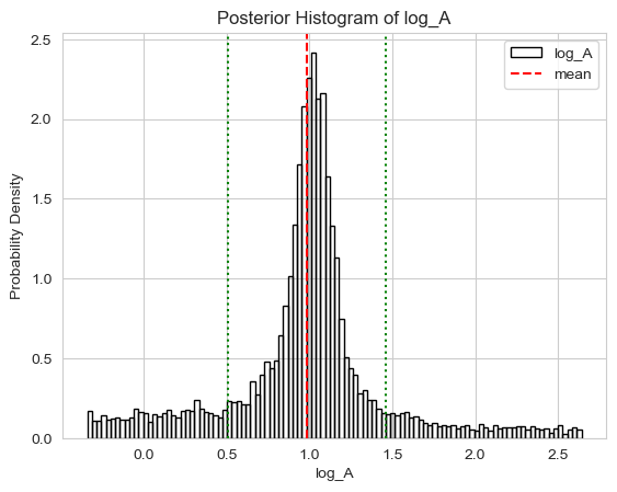
get_evidence: Returns the evidence of the modelprint_summary: Prints the summary of the Nested Sampling run.plot_cornerplot: Plots the corner plot of the posterior distribution.posterior_plot: Plots the posterior distribution of given parameter.comparison_plot: Plots the samples of two parameters against each other.get_max_posterior_parameters: Returns the Maximum a posteriori parametersget_max_likelihood_parameters: Returns the Maximum Likelihood parameters
The Demonstration notebook to be attached with the Stingray Notebooks repository is : Notebook
Future Work
Future Work in continuation of this project will be:
1) Improving the Documentations for various functions and classes in the PR.
2) Adding more Kernel and Mean Models to the code for other use cases.
3) Adding example Notebooks to the Stingray Notebooks repository demonstrating the tools use on various Datasets.
4) Importantly, updating the code based on the feedback from the Astronomy community.
Libraries Used
The External libraries used in this project are:
1) JAX
The Jax python library was used as the primary backend, as it can combine functional programming with potent array operations, making it ideal for scientific tasks and machine learning. Key features are Jax.grad for derivatives, Jax.jit for code compilation, and Jax.vmap for efficient batching.
2) Tinygp

The TinyGP Python package was used for Gaussian Processes (GPs) backend as it offers essential functionalities for modeling and inference with GPs, including covariance functions, hyperparameter optimization, and predictive uncertainty estimation. The package is written in Jax so it is compatible with our backend and most essentially it has the kernels we are using in an optimised form.
3) Jaxns
The Jaxns Python package was used for Nested Sampling backend as it offers a simple and efficient way to perform Nested Sampling. It’s built using JAX, enabling the entire inference process to be translated into XLA primitives for efficient, high-performance JIT compilation. It also has a very simple API, which makes it easy to use and integrate with our other libraries.
4) Tensorflow_Probability
Apart from these libraries I also used tensorflow_probability for the priors, as it has a wide range of distributions and is compatible with Jax.
Maths Behind the Project:
This project deals with Bayesian inference for the calculation of Bayes factors to characterize model preference and thereby the significance of QPOs within time series data,
To understand the meaning of Bayes factors, we consider Bayes’ theorem
\[p(\theta \| D, M) = \frac{p(D \| \theta, M ) p(\theta \| M)}{Z(d \| M)}\]
The parts of this expression in brief:-
- \(p(\theta \| d, M)\): The posterior probability of the parameters over the data for the model M
- \(\pi ( \theta \| M)\): The prior probability of the parameters of the model M
- \(L(d \|\theta , M)\): The likelihood of the data given the parameters of the model M
- \(Z(d \| M)\) : Evidence, The probability of the model to give the Data
All these probabilities are conditioned on the combined Kernel and Mean Model M (GP Model), which we want to evaluate. The evidence describes an overall probability of the given model producing the data, and can be calculated by rearranging and integrating Bayes’ theorem:
\[Z(D \| M ) = \int_{}{} p(D \| \theta, M ) p(\theta \| M) d \theta\]
The evidence is expensive to solve using Grid methods or Monte Carlo integrals, hense we use sophisticated method like Nested Sampling. Though the evidence itself carries no straightforward intrinsic meaning as a normalization factor, taking the ratio between two yields the Bayes factor
\[BF = \frac{Z(D \| M_1 )}{Z(D \| M_2 )}\]
where M_1 and M_2 are the different models that yield the respective evidences. The Bayes factor measures the odds of the underlying data being produced by either model, assuming both models are equally likely to be correct, though it does not measure if the model itself is a good fit to the data.
This is essentially what we are targetting for our evaluation. We take 2 Models, one with a QPO kernel (hense QPO behaviour) and one with only Red Noise and compare the Bayes Facotrs of the both Models to produce the data, helping us determine whether the Time Series has a QPO or not. Also, by doing posterior sampling, if the Bayes Factor is high enough, we can get the posterior distribution for the QPO frequency and other parameters which are directly linked to the physics of these events.
The models that we are using are Gaussian Process (GP) models which are charachterised entirely by their kernel function and mean function. For example,
A QPO plus RN kernel looks like (where \(\tau = abs(t_i- t_j)\).):
\[k_{qpo+rn} = a_{qpo} exp(-c_{qpo} \tau)cos(2 \pi f_{qpo}) + a_{rn} exp(-c_{rn})\]
A Gaussian mean for the model can be written as:
\[\mu_{gauss} = A exp(-\frac{(t-t_0)^2}{2\sigma^2})\]
Astronomy Behind the Project:
Analysis of Quasi Periodicities is important in understanding the dynamic of many Astrophysical objects during transient events like:
1) Gamma Ray Bursts:
 GRB: Hypernova Collapse (Image Source)
Gamma-ray bursts (GRBs) are extremely energetic and intense bursts of gamma-ray radiation that originate from distant regions of space. They are the most explosive events in the universe. GRBs come from so far and are yet so powerful that even Supernova explosions could not explain them. These could only be caused by a focused beam like expulsion of energy.
There are two main types of GRB’s : Long and Short duration bursts.
The cause for the Long Duration GRB’s (> 2 secs ) are the collapse of massive stars, which are 20 to 30 times the mass of the Sun (also called Hypernova). When the core of such a massive star collapses, forming a Black Hole, the material just outside the core falls down into it, forming a swirling hot Accretion Disk around the Black Hole. The magnetic field lines of the Black Hole gets coiled and the energy is released in the form of a jet of radiation, which is focused in a narrow beam. (EG: GRB 050724)
The Video is for the Gamma Ray Burst of GRB 080319B was aimed almost precisely at the Earth, which made it the brightest gamma-ray burst observed to date by NASA’s Swift satellite. (Source NASA)
 GRB: Neutron Star Merger (Image Source)
The cause for the Short Duration GRB’s ( \(\sim\) milisecs) is Two Neutron Stars or a Neutron Star and a Black Hole crashing together and Exploding (also known as Kilonova). These massive objects while revolving around each other, lose energy by radiatiing away Gravitational Waves (quite literally ripples in Fabric of space time). These stars draw closer and closer to each other for Billions of years and when up close they spin exteremely rapidly. If their combined mass is more than 2.8 Solar masses, they will collapse to form a Black Hole. This Black Hole and Neutronium debri system then proceeds to form an accretion disk and blasting out a GBR. As the material is much more compact, the flash is much shorter. (Credits: NASA) (Also, EG: GRB 050328)
QPO Flux: Quasi Periodic Oscillations in GRB’s are yet to be confirmed. Experimenters use tools like ours to try and find evidences of QPO’s while theorists are try to find possible models which could cause such a behaviour (Leading theories use the lense thirring effect).
(Source: Ziaeepour, H., & Gardner, B. 2011, Journal of Cosmology and Astroparticle Physics)
GRB detections are rare as they need to be pointed in our direction to be visible to us. They are also very short lived, so we need to be looking at the right place at the right time. Fortunately, we have help from another field of Astronomy, Gravitational Wave Astronomy. These mergers release insane amount of Gravitational Waves, which are detected by LIGO and Virgo detectors.
These detectors can tell us the direction of the source, which can then be observed by telescopes. This is how we detected the first Neutron Star merger, GW170817, which was also the first time we detected both Gravitational Waves and Electromagnetic Radiation from the same event. (Source: NASA). With more and more Gravitational Wave detectors coming online, we can expect to narrow down their loaction and use both the Electromagnetic and Gravitational Waves data to completely understand the dynamics of these mergers (Also, hopefully uncover new Physics :)).
GRBS are the most epic events in the Universe (literally visible Halfway through the Universe), they are the birth cries of Black Holes being born, and working on them in this project was a very exciting experience.
2) Giant Magnetar Flares:
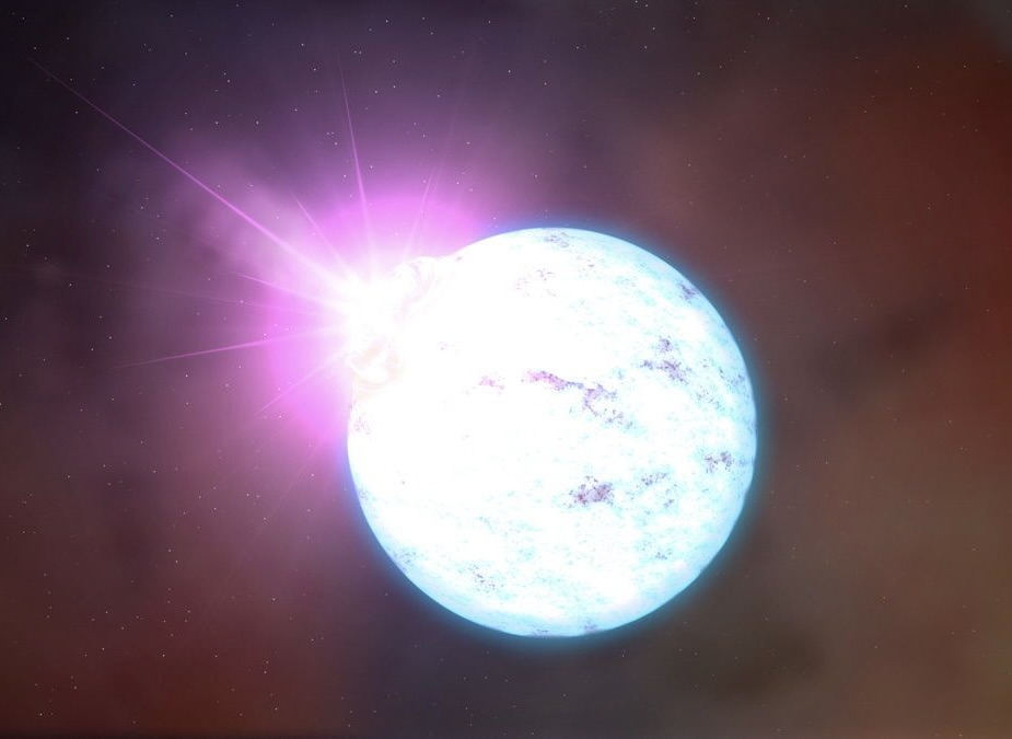 Magnetar Flare (Image Source)
Pulsars are rapidly rotating Neutron Stars, which coupled with their strong magnetic field launches two opposite beams of Electromagnetic Radiation. These beams sweep around as the star moves and we on earth see it as a pulse of increased brightness in lightcurves.
Magnetars are a special class of Pulsars with extremely strong magnetic fields. They are rarer and have short lifetimes, as their intense magnetic fields slow down their spinning rate over time (also weakening the field).
They are known to emit short bursts of X-Rays and Gamma Rays called Giant Magnetar Bursts. The most widely believed theory is that these bursts are caused by the with magnetic coupling of the crust to the core.
In the Neutron Star, the Crust and the Magnetic Field are locked together so a change in one affects the other. The crust of the star is under incredible strain due to the intense gravity and rapid rotation. When the crust reaches its breaking point, it can crack and release energy in the form of a flare. This process might be similar to earthquakes on Earth and is called a star quake.
 Magnetar Burst Clip (Image Source)
In a fraction of a secound a Mangnetar can release more energy than the Sun can in a quater million years. This radiation is majorly in the X and Gamma Ray Spectrum. SGR 1806-20 is a magnetar in our galaxy, which released a burst of gamma rays in 2004, which was so powerful that it was detected by the earth’s atmosphere, despite being 50,000 light years away. (Source: NASA Swift)
QPO Flux: Neutron Star Seismology explains the Observed QPO frequencies to be related to the torsional shear oscillations of the solid crust of a neutron star excited during a giant flare event. Latest Models however suggest that the magnetic field dampens the crust oscillations and we actually observe long-lasting QPO’s in the fluid core of the magnetar.
(Source: Magneto-elastic oscillations and the damping of crustal shear modes in magnetars, Michael Gabler, Pablo Cerda-Dur, Monthly Notices of RAS)
3) Solar Flares:
 Solar Flare (Image Source)
Solar flares are sudden, intense bursts of energy and radiation emanating from the Sun’s surface.
The Magnetic Field lines on the Sun’s Surface, have a huge amount of energy stored in them. Often these field lines get tangled up, and if the conditions are right, they can snap creating a gigantic Short circuit. All the energy stored in the field lines is released at once, creating a Solar Flare. A big solar flare can release as much as 10% of the entire Suns energy output.
These eruptions emit a broad spectrum of electromagnetic radiation, including X-rays and ultraviolet light, and also solar material and Neutrinos. Solar flares are classified into different categories based on their strength, with X-class flares being the most powerful. Studying solar flares helps us understand solar activity, space weather, and the dynamic interplay between magnetic fields and plasma on the Sun’s surface.
QPO Flux: Quasi Periodic Pulsation have been observed in Solar flares for half a century. The leading solar models point to the presence of magnetohydrodynamic (MHD) oscillations in coronal structures (magnetic loops and current sheets) or quasi-periodic regimes of magnetic reconnection to explain this Quasi Periodic Flux.
(Source: Quasi-Periodic Pulsations in Solar and Stellar Flares, I. V. Zimovets, J. A. McLaughlin, Springer)
4) X-Ray Binaries:
X-ray binaries are binary star systems in which one of the stars is a compact object, such as a black hole (usually Quasars: Extremely luminous galactic cores where gas and dust falling into a supermassive black hole emit a beam of electromagnetic radiation) or a neutron star, while the other is a normal star like the Sun or a massive star.
 Accretion Radiation (Image Source)
The compact object accretes material from its companion star, creating a disk of hot, high-energy gas around it. This accretion process releases a significant amount of X-ray radiation, which makes these systems observable in X-rays. Compared to the above mentioned events related to Black Holes and Neutron Stars, this one is relatively less explosive (relatively).
X-ray binaries are crucial in studying the properties of compact objects, as they provide insights into their masses, sizes, and accretion processes. They also serve as laboratories for testing theories of strong gravity and high-energy physics. Observing X-ray binaries helps astronomers learn about the interactions between stars, the behavior of matter in extreme environments, and the evolution of binary systems.
QPO Flux: Black hole and neutron star X-ray binary systems routinely show quasi-periodic oscillations (QPOs) in their X-ray
flux. These QPO pulsations are now thought to be produced due to the Lense Thirring Effect. This is a relativistic effect
whereby a spinning massive object twists up the surrounding spacetime, strring the accreting flows and creating Quasi Periodic radiations. These contain Type A,B, and C for low freq QPO’s (freq < 30 Hz) and other High freq QPO’s (freq > 60 Hz)
(Source: A review of quasi-periodic oscillations from black hole X-ray binaries: Observation and theory Adam R. Ingram
,Sara E. Motta Astronomy Reviews)
Challenges and learnings
1) Software Development is not only about implementing some algorithm
I was drawn to this project as it was using cutting edge Bayesian Analysis Methods (a part I like Mathematically) to analyse Extremely violent Events in the Universe (Something I find very interesting). This led me to believe that in this project, I have to write a code to implement the GP and Evidence Calculation Algroithm and use it to analyse some data.
I could’nt have been more wrong. This project in my opinion was more about making a suitable interface for the user to use the code, and making the code robust enough to handle all the different use cases. Which classes to make, which functions to use, where to give flexibilty and where to Hard Code? These were the questions that I spent the most time answering and I kept on changing my code based on these.
2) The Importance of Documentation
While working on this project, I had to use a lot of different libraries and I realised that the documentation for these libraries is not always good (or maybe I am a bit too begineer level to not understand obvious things :) ). I had to go through the source code of these libraries to understand how to use them, and I realised that I should write good documentation for my code, so that other people don’t have to go through the same trouble.
3) Code and Compatability
In any program, we always make some package imports. Now these packages may have been written some time ago, and some times what you want to do with their code is quite different to what the developers had taken into account during the design, so your code breaks.
This happened to me with JAX while making the windowed likelihood function. The plan was that the whole lightcurve may not have a QPO, and in that case, we will create a window (tmin to tmax), so that we consider that part to have the QPO, and the rest of the part was White Noise. Now, as it happened, Jax is a functional programming language and so it must know the sizes of all the arrays in the computation, but here we were slicing the lightcurve into undeterministic size (tmin and tmax are random variables).
I had to give up after a lot of tries and documentation searches, showing that people might use your code in very different ways than you had intended.
4) The importance of Testing
The importance of Code Testing has been stressed upon by many developers, and I now have a first hand account of how important it is as any change I would make, however small would definitely break some test cases. This made me realise that your code is a small but complicated part of a big and complicated system, and breakdowns are bound to happen and adequate Testing is the best way to ensure that the system is working as intended.
5) The Wonderful Open Source Community
When people think of Open Source they think of Code that is available for all to see, rather than private code, but reality cannot be any more further than that!! Open Source is all about collaboration. I learned this the nice way in this project.
Firstly I was having some difficulty implementing my conditioned beta priors using Tensorflow Probability distribution and was finding it difficult to find it up in the documentation. So I thought that perhaps, I might get some hints if I ask in the email channel, and guess what, the maintainers not only replied back fast, they gave me a well written explaination, and links for further reference.
Secoundly, I also had to implement some prior functions in the Jaxns prior model, so on the advice of my mentors, I wrote a issue in the library, and this started a very enjoyable interchange between me and the library author . I would ask a question at the night, and when I would wake up I would have a well written reply.
Such experiences with so many amazing people has made realise the real meaning of Open Source, and you bet I will be recipocating all this help to other programmers.
Blogs
These are the blogs I wrote during the project detailing my work, challenges and progress in the project;
-
What is the Community Bonding Period?
-
My adventure with the implementation
-
Starting the implementation
-
Making a Demo
-
Pull request made
Acknowledgements
I would like to end by thanking my Mentors, Daniela Huppenkothen and Matteo Bachetti, for their encouragement and support during this project. Their patience with my mistakes and offhand solutions to my issues were very helpful in it.
Lastly I would also like to thank the Google Summer of Code program for giving me the opportunity to work on this project and learn so much from it.