5.1. Basic Probability

Here we will look at the definitions and meaning of some important concepts in Probability Theory

5.1.1. Random Variable

A random variable, usually written X, is a variable whose possible values are numerical outcomes of a random phenomenon. There are two types of random variables, discrete and continuous.

The range space of a discrete RV is discrete, while for a continuous RV it is continuous. Discrete RV’s have a probability distribution whereas continous RV’s have a probability density function

Probability theory works on random variables, and all definations examples are best understood in this framework

Symbols: $X$ for the RV, $x$ for its value, $f_X(x)$ for its pdf. ($P_X(x)$ for discrete)

5.1.1.1. Cdf

Cdf (cumulative density function) of a Random variable X is denoted by $F_X(x)$.

The cdf at x is the probability that if we sample/measure X, its value will be less than x.

$$F_X(x)=P(X\le x)$$

Cdf functions can be calculated by:-

• Discrete: $F_X(x)=\sum _{K\le x}{P}_x(k)$

• Continuous: $F_X(x)={\int }_{-\mathrm{\infty }}^x{f}_X(t)dt$

Quantile: $q_X(t)=F_X^{-1}(t)$, or the inverse of cdf function gives us the value of x before which the probabilty is t, and is useful in MCMC methods, simulations.

5.1.1.2. Multiple Random variables

For the case of two random variables, let the RVs be $X,Y$, and the values be $x,y$. The various probabilities for the two will be:-

a. Joint pdf:

$$f_{X,Y}(x,y)=P(X=x,Y=y)$$

Joint probability of both variables having a specific value

b. Marginal pdf:

$$f_X(x)={\int }_{-\mathrm{\infty }}^{+\mathrm{\infty }}{f}_{X,Y}(x,y)dy$$

the probabilty of the random variable X having value x, if we have not observed y. Ie, pdf of X if we have the joint pdf

c. Conditional pdf:

$$f_{X,y}(x,y)=\frac{f_{X,Y}(x,y)}{f_X(x)}$$

Probability of RV X having a value x, conditioned on some value y for RV Y. The denominator is for normalisation.

Similary this can be extended to more than two multiple random variables

5.1.2. Expection, Variance, Moments

Expectations are weighted averages of functions of random variables, where the weights are the pdf of the random variable and the values are values of the random variable.

The expected value of a function $g(x)$ of a continous random variable X with pdf $f_X(x)$ is:

$$\mathbb{E}[g(X)]={\int }_{-\mathrm{\infty }}^{+\mathrm{\infty }}g(x)f_X(x)dx$$

It means that if X is a RV then $\mathbb{E}[g(X)]$ is the average value we get when we sample the transformed value $g(X)$ many times. Note:

1. Any transformation of a RV is also a RV, hense here g(X) is also a RV.

2. The pdf if the weight as more the pdf more probabilty of that value occuring

3. The fact that we sample many times leads to a useful estimate of $\mathbb{E}[g(X)]$

It does not mean the expected value of the RV so never say that, rather it is always reffered to as the expectation value

Means

The mean or the first moment of a Random Variable is given by:

$${\mu }_X=\mathbb{E}[X]={\int }_{-\mathrm{\infty }}^{+\mathrm{\infty }}x{f}_X(x)dx$$

Also, the $r^{th}$ moment is given by:

$$\mathbb{E}[X^r]={\int }_{-\mathrm{\infty }}^{+\mathrm{\infty }}{x}^r{f}_X(x)dx$$

5.1.2.1. Variance

Variance of any RV X is its secound central moment defined by:

$$Var(X)=\mathbb{E}[(X-\mathbb{E}{)}^2]={\int }_{-\mathrm{\infty }}^{+\mathrm{\infty }}(x-{\mu }_X{)}^{2}f(x)dx$$

After some calculations, we can simplify it to:

(5.1)$$\begin{array}{rl}Var(X)& =\mathbb{E}[X^2+{\mathbb{E}}^2-2X\mathbb{E}]\\ & =\mathbb{E}[X^2]+(\mathbb{E}[X]{)}^2-2\mathbb{E}[X]\mathbb{E}[X]\\ & =\mathbb{E}[X^2]-(\mathbb{E}[X]{)}^2(imp)\\ & =\mathbb{E}[X^2]-({\mu }_X{)}^2\\ & ={\int }_{-\mathrm{\infty }}^{+\mathrm{\infty }}{x}^2{f}_X(x)dx-({\mu }_X{)}^2\end{array}$$

5.1.2.2. Multiple Random Variables

Expectation Value of the product of two random variables is given by:

$$\mathbb{E}[XY]={\int }_{-\mathrm{\infty }}^{+\mathrm{\infty }}{\int }_{-\mathrm{\infty }}^{+\mathrm{\infty }}xy{f}_{X,Y}(x,y)dxdy$$

Covariance of X,Y is given by:

$${\sigma }_{X,Y}=cov(X,Y)=\mathbb{E}[(x-{\mu }_X)(y-\mu (Y))]=\mathbb{E}[XY]-{\mu }_X{\mu }_Y$$

Coorelation of X,Y is given by:

$$\rho (X,Y)=correlation(X,Y)=\frac{cov(X,Y)}{\sqrt{Var(X)Var(Y)}}=\frac{{\sigma }_{X,Y}}{{\sigma }_X{\sigma }_Y}$$

the correlation actually has a meaning between the physical relations of the two radom varaibles, as to how they vary with each other.

5.1.2.3. Independence:

Two random variables X and Y can be called independent if $f_{X,Y}(x,y)=f_X(x)f_Y(y)$ (Note: having 0 correlation does not imply independence).

Which means that if $p(X=x,Y=y_i)=p(X=x,Y=y_j)$ (for all i,j) , ie the probability is independent of the value of Y then X and Y are independent RVs.

A set of multiple Random Variables $\{X_1,X_2,...X_n\}$ is independent if:

$$f(x_1,...x_n)=\prod _{j=1}^n{f}_j(x_j)$$

5.1.3. Random Sample

Let X be a random variable with pdf $f_X(x)$, then a random sample from X is a set of random variables $\{X_1,X_2..X_n\}$ if they are sampled out of X.

$X_i=i^{th}$ random sample (a RV), $x_i=$ value of the $i^{th}$ random sample.

A set of random samples is set to be independent and identically distributed (iid) if:

$$f(x_1,...x_n)=\prod _{i=1}^n{f}_X(x_i)$$

5.1.4. Properties of Expectation and Variance

1. $\mathbb{E}[aX+b]=a\mathbb{E}[X]+b$ : Expectation of Linear transform of a RV’s

2. $\mathbb{E}[X+Y]=\mathbb{E}[X]+\mathbb{E}[Y]$ : Expectation of adding two different RV’s adds both.

(5.2)$$\begin{array}{rl}{\int }_{-\mathrm{\infty }}^{\mathrm{\infty }}{\int }_{-\mathrm{\infty }}^{\mathrm{\infty }}(x+y)f_{X,Y}(x,y)dxdy& ={\int }_{-\mathrm{\infty }}^{\mathrm{\infty }}x{\int }_{-\mathrm{\infty }}^{\mathrm{\infty }}(y)f_{X,Y}(x,y)dydx+{\int }_{-\mathrm{\infty }}^{\mathrm{\infty }}y{\int }_{-\mathrm{\infty }}^{\mathrm{\infty }}(x)f_{X,Y}(x,y)dxdy\\ & ={\int }_{-\mathrm{\infty }}^{-\mathrm{\infty }}x{f}_X(x)dx+{\int }_{-\mathrm{\infty }}^{-\mathrm{\infty }}y{f}_Y(y)dy\end{array}$$

3. $\mathbb{E}[XY]=\mathbb{E}[X]\mathbb{E}[Y]$, : If X,Y are independent RVs

4. Var(a) = 0 : Variance of a scalar is zero

5. $Var(aX+b)=a^{2}Var(X)$, as $\mathbb{E}[(aX-\mathbb{E}[aX]{)}^2]=a^2\mathbb{E}[(X-\mathbb{E}[X]{)}^2]$

Variance of Linear Transformation of a RV

6. $Var(X+Y)=Var(X)+Var(Y)-2Cov(X,Y)$, : Variance of Sum of two RV’s

Proof:

(5.3)$$\begin{array}{rl}Var(X+Y)& =\mathbb{E}[(x+y-\mathbb{E}[X+Y]{)}^2]\\ & =\mathbb{E}[((x-{\mu }_X)+(y-{\mu }_Y){)}^2]\\ & =\mathbb{E}[(x-{\mu }_X{)}^2]+\mathbb{E}[(y-{\mu }_Y{)}^2]+\mathbb{E}[2(x-{\mu }_X)(y-\mu Y)]\\ & =Var(X)+Var(Y)-2Cov(X,Y)\end{array}$$

7. For random samples: if $\{X_1,X_2,...X_n\}$ are iid, then

$$\mathbb{E}[X_1+X_2+...X_n]=n{\mu }_{X}Var(X_1,X_2,...X_n)=n({\sigma }_X{)}^2$$

For the sample mean is $\overline{X}=\frac{1}{n}\sum _{i=1}^n{X}_i$, the expectation value and variance is

$$\mathbb{E}[\overline{X}]={\mu }_X,Var(\overline{X})=\frac{{\sigma }_X^2}{n}$$

Proof:

(5.4)$$\begin{array}{rl}Var(\overline{X})& =Var(\frac{1}{n}(X_1+X_2....X_n))\\ & =\frac{1}{n^2}Var(X_1+X_2+...)\\ & =\frac{n}{n^2}Var(X)\end{array}$$

as $Var(\overline{X})=Var(\frac{1}{n}(X_1+X_2....X_n))=\frac{1}{n^2}Var(X_1+X_2+...)=\frac{n}{n^2}Var(X)$,

here, we have independent samples

Note: in the important case that we will study ie. MCMC, the sample will not be independent.

5.1.5. 3 Fundamental Laws

5.1.5.1. Weak Law of Large Numbers (WLLN)

The Weak Law of Large Numbers states that the sample mean converges in probability to the population mean.

Suppose ($X_1,X_2,...X_n$) are independent and identically distributed random numbers picked from a RV X.

Then, for every $ϵ>0$,

$$\underset{n\to \mathrm{\infty }}{lim}P(|{\overline{X}}_n-\mu |<ϵ)=1$$

5.1.5.2. Strong Law of Large Numbers (SLLN)

The Strong Law of Large Numbers states that the sample mean converges almost surely to the population mean.

That is, for every $ϵ>0$,

$$P(\underset{n\to \mathrm{\infty }}{lim}|{\overline{X}}_n-\mu |<ϵ)=1$$

5.1.5.3. Central Limit Theorem (CLT)

Probabilty distribution (pdf) of the sample mean $\overline{X}$ of a RV $X$ tends to a normal distribution, with mean ${\mu }_X$, and variance $\frac{{\sigma }_X^2}{n}$ as we increase the size of the sample. All the higher moments and central measures tend to zero as n tends to infinity

Also stated as:

If ($X_1,X_2,...X_n$) is a random sample from a distribution with mean $\mu$, and finite variance ${\sigma }^2>0$, then the limiting distribution of

$$Z_n=\frac{\overline{X}-\mu }{\sigma /\sqrt{n}}$$

is the standard distribution.

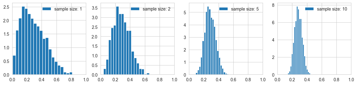
Here we will try a small example and see the central limiting tendency of sample mean for a Beta(2,5) pdf.

# Take a double normal and make histograms of samples of means of random samples of size 1,2,5, 10

import numpy as np
import matplotlib.pyplot as plt
import seaborn as sns
sns.set_style('whitegrid')

sample_mean_sizes = [1, 2, 5, 10]

# Set up the figure
fig, ax = plt.subplots(1, 4, figsize=(14, 3))

# Using a beta distribution with alpha = 2, beta = 5

# Plot the samples
for i, sample_mean_size in enumerate(sample_mean_sizes):
    sample_means = []
    for j in range(2000):
        sample = np.random.beta(2, 5, sample_mean_size)
        sample_means.append(np.mean(sample))
    ax[i].hist(sample_means, bins = 20, density = True, label='sample size: ' + str(sample_mean_size) )
    ax[i].set_xlim(0, 1)
    ax[i].legend(loc='best', frameon=False)

plt.show()