3.1. Basic MCMC

Let us try to do an experiment to evaluate the maximum of a function f(x).

What we will do is, we will start from a point (\(x_0\)) and then make jumps according a random function (say U(0,1)). We will make the jump to the next point if

\[ random(0,1) < \frac{f(x_{i})}{f_{i-1}} \]

Ie, if the next point is higher then will jump to else we will jump based on the fraction of both values vs a Uniform number in (0,1).

As it turns out this method works very well even compared to Stochastic Gradient Descent, as we are constantly progressing to the maxima, but still have randomness with us to bail us out of sticky situations.

As, we will also see, this Monte Carlo Walker actually makes a tour of the parameter space and visits volumes proportional to the function values at those points (have to take the volume element also into account, see High dimensional data chapter).

This is also the basis of the Monte Carlo Methods for parameter sampling.

3.1.1. Monte Carlo Walker

Making the plot of markov chain walker, and analysis its path

# Importing Dependencies
import numpy as np
import matplotlib.pyplot as plt
import seaborn as sns
from jax import random, grad, vmap
import jax.numpy as jnp

sns.set_style('whitegrid')

# Making a monte carlo walker (optimiser) for a function
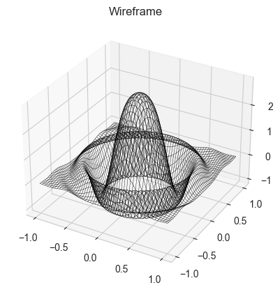
def simplef1(x,y):
    return 3*jnp.cos(((3*x)**2+(3*y)**2))*jnp.exp(-3*(x**2+y**2))

x = jnp.linspace(-1,1,200)
y = jnp.linspace(-1,1,200)
X,Y = jnp.meshgrid(x,y)
Z = simplef1(X,Y)

fig = plt.figure()
ax = plt.axes(projection = '3d')
ax.plot_wireframe(X,Y,Z,color = 'black', lw = 0.3)
ax.set_title('Wireframe')

Text(0.5, 0.92, 'Wireframe')

# Doing monte carlo walking on this function:-
x0 = 0.8; y0 = 0.8
n = 200

def monte_carlo_walk(fun, x0, y0, n, bounds = (np.array([-2,2]) ,np.array([-2,2])) ):
    xs = np.zeros(n); ys = np.zeros(n)
    for i in range(n):
        x1 = 0.2*random.normal(random.PRNGKey(i),shape = (1,)) + x0
        y1 = 0.2*random.normal(random.PRNGKey(i+1),shape = (1,)) + y0
        if (x1 < bounds[0][0]) or (x1 > bounds[0][1]) or (y1 < bounds[1][0]) or (y1 > bounds[1][1]):
            x1 = x0
            y1 = y0
            i = i-1
            continue
        if fun(x1,y1) > fun(x0,y0):
            x0 = x1
            y0 = y1
        else:
            flip = random.uniform(random.PRNGKey(i+2),shape = (1,))
            if flip < fun(x1,y1)/fun(x0,y0):
                x0 = x1
                y0 = y1
            else:
                x0 = x0
                y0 = y0
        xs[i] = x0; ys[i] = y0
    return xs, ys

fig = plt.figure()
xs, ys = monte_carlo_walk(simplef1, x0, y0, n)
ax = plt.axes(projection = '3d')
ax.plot_wireframe(X,Y,Z,color = 'black', lw = 0.3)
ax.scatter(xs,ys,simplef1(xs,ys),color = 'blue',s = 5)
ax.plot(xs,ys,simplef1(xs,ys),color = 'red',lw = 0.5)
ax.set_title('Monte Carlo Walk')

Text(0.5, 0.92, 'Monte Carlo Walk')

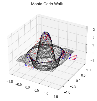
Why will gradient descent fail here?

Gradient Descent is likely to fail if the Hyperparameter tuning is not done properly, as the sfunction is symmentric and has many local maximas, which can make the process stuck in a local mode.

We also claimed that the walker will trace out the function based on its values at different points, hense we will take 10000 points and show that the histogram formed resembles the function

xs, ys = monte_carlo_walk(simplef1, x0, y0, 20000)

def plot3dhist(xs, ys, starts, ends, bins):
    z_hist = np.zeros((bins[0]+1, bins[1]+1))
    for i in range(len(xs)):
        z_hist[int((xs[i]-starts[0])/(ends[0]-starts[0])*bins[0])-1, int((ys[i]-starts[1])/(ends[1]-starts[1])*bins[1])-1] += 1

    x = jnp.linspace(starts[0],ends[0], bins[0]+1)
    y = jnp.linspace(starts[1],ends[1], bins[1]+1)
    X,Y = jnp.meshgrid(x,y)
    Z = z_hist/len(xs)
    fig = plt.figure()
    ax = plt.axes(projection = '3d')
    ax.plot_wireframe(X,Y,Z,color = 'black', lw = 0.3)
    ax.set_title('Wireframe')
    plt.show()

# plot3dhist(xs[5000:9999],ys[5000:9999],[-2,-2],[2,2],(50,50))
plot3dhist(xs,ys,[-2,-2],[2,2],(50,50))

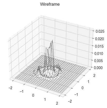
This took almost 20 s to run on my computer, for such a simple implementation (although it uses a lot of for loop). This makes us appreciate how much powerful our methods have to be if we have to work on complex distributions with thousands of parameters and many complicated priors.

#  Finding Gradient
def simplef12(w):
    x = w[0]; y = w[1]
    return 3*jnp.cos(((3*x)**2+(3*y)**2))*jnp.exp(-3*(x**2+y**2))

gradient = grad(simplef12)(jnp.array([0.8,0.8]))
print(gradient)

[0.6487649 0.6487649]

One can see, that as the function is symmetric, the gradient will also be, and this may easily get stuck if started farther from 0

3.1.2. Basics of markov chains

The above monte carlo walker seems to be efficiently travelling along the target function in proportion to the function values. If we have a probability distribution that we have to sample then, this seems like a good method as it only requires that we can get the value at any point on the function. But why does it work?

The reason being that the methods forms a set of stochastic variables known as a Markov chain, whose stationary distribution is equal to the target distribution.

A Markov chain or Markov process is a stochastic model describing a sequence of possible events in which the probability of each event depends only on the state attained in the previous event.

\[ P(X_{t+1} = X^{t+1} | X_{t} = X^{t}, X_{t-1} = X^{t-1}, X_{t-2} = X^{t-2}, ... ) = P(X_{t+1} = X^{t+1} | X_{t} = X^{t}) \]

here \(X_{t}\), is the t’th element of the chain of random variables

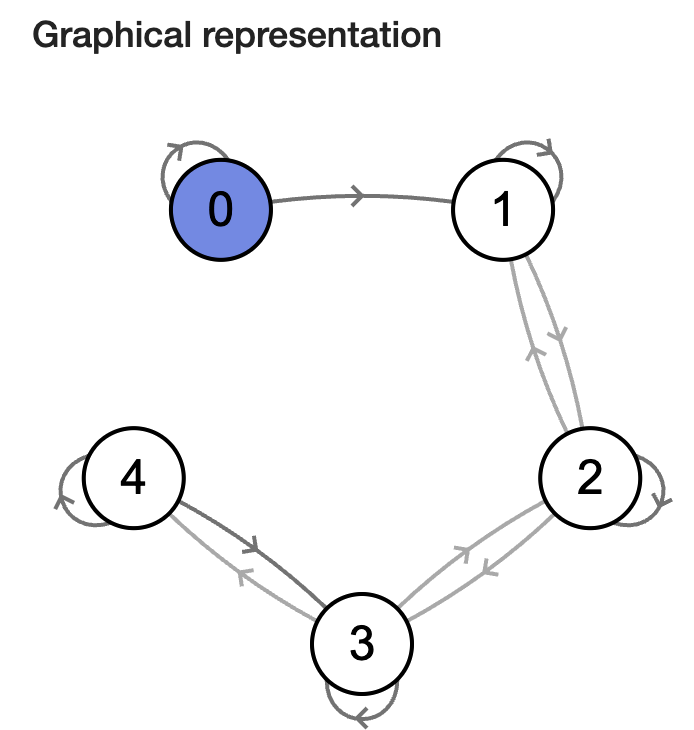
Fig. 3.1 Markov chain diagram.

To simplify, let us take an example of a chain with discrete, finite range. Suppose a person takes a random walk on a number line on the values 1, 2, 3, 4, 5. If the person is currently at an interior value (2, 3, 4), in the next second she is equally likely to remain at that number or move to an adjacent number. If she does move, she is equally likely to move left or right. If the person is currently at one of the end values (1 or 5), in the next second she is equally likely to stay still or move to the adjacent location.

This is a simple discrete Markov chain, as the probability of the girl going to any place in next step depends on only her current position. (Discrete as the chain is discrete random variables, not because of the range space). We can describe her movements in terms of transition probabilities in a matrix P where

\( P_{i,j} = prob\)(transitioning from state \(X_{i}\) to \(X_{j}\))

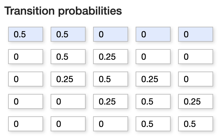
Fig. 3.2 Transition Matrix.

Credits: http://markov.yoriz.co.uk/

3.1.2.1. Some Important Features

1. Irreducible Markov Chain: A markov chain in which each point is reachable from any other point in finite number of steps

2. Periodic Markov Chain: A chain which can return to the same state only in regular intervals of time. (Chain length)

3. Reccurent Markov Chain: A chain is said to be recurrent if, any time that we leave any state, we will return to that state in the future with probability one. On the other hand, if the probability of returning is less than one, the state is called transient.

We represent one’s current location as a probability row vector of the form: \(p = (p_{1}, p_{2}, p_{3}, p_{4}, p_{5})\) where \(p_{i}\) represents the probability that the person is currently in state i .

If \(p^{j}\) represents the location of the traveler at step j, then the location of the traveler at the j+1 step is given by the matrix product: \(p^{j+1} = p^{j} P\), and hense the probability vector after travelling m steps will be:

\[ p^{j+1} = p^{j} P^{m} \]

STATIONARITY

For an irreducible, aperiodic Markov chain, there is a limiting behavior of the matrix power \(P^{m}\) as m approaches infinity. Specifically, this limit is equal to

\[ W = \lim_{m \to \infty} P^{m} \]

The implication of this result is that, as one takes an infinite number of moves, the probability of landing at a particular state does not depend on the initial starting state.

From this result about the limiting behavior of the matrix power \(P^{m}\), one can derive a rule for determining this constant vector. Suppose we can find a probability vector w such that \(w = wP\). This vector w is said to be the stationary distribution. If a Markov chain is irreducible and aperiodic, then it has a unique stationary distribution. Moreover, as illustrated above, the limiting distribution of this Markov chain, as the number of steps approaches infinity, will be equal to this stationary distribution.

# Simulating relative frequencies of a markov chain random walker
from numpy import random as npr
npr.seed(16)

steps = 5000
probs = np.zeros((5,steps))
P = np.array([[0.5,0.5,0.0,0.0,0.0],[0.25,0.5,0.25,0.0,0.0],[0.0,0.25,0.5,0.25,0.0],
              [0.0,0.0,0.25,0.5,0.25],[0.0,0.0,0.0,0.5,0.5]])

pstart = np.array([0.0,0.0,0.0,1.0,0.0])
state = 3
probs[:,0] = pstart

for i in range(steps-1):
    u = npr.uniform(0,1)
    if state == 0:
        if u < 0.5: state = 0
        else: state = 1
    elif state == 1:
        if u < 0.25: state = 0
        elif u < 0.75: state = 1
        else: state = 2
    elif state == 2:
        if u < 0.25: state = 1
        elif u < 0.75: state = 2
        else: state = 3
    elif state == 3:
        if u < 0.25: state = 2
        elif u < 0.75: state = 3
        else: state = 4
    else:
        if u < 0.5: state = 3
        else: state = 4
    probs[state,i+1] = 1
    probs[:,i+1] = (probs[:,i])*(i/(i+1)) + (1/(i+1))*probs[:,i+1]

fig, ax = plt.subplots(1, 5, figsize =(13, 3))
x = np.linspace(1,steps,steps)
for i in range(5):
    ax[i].plot(x,probs[i,:])
    ax[i].set_title('State '+str(i))
    ax[i].set_ylim([0.0,0.5])
    if (i == 0) | (i == 4):
        ax[i].axhline(y = 0.125, color = 'red', linestyle = '--')
    else:
        ax[i].axhline(y = 0.25, color = 'red', linestyle = '--')
    if (i == 0):
        ax[i].set_ylabel('Relative Frequency')

# Lets run a code and see what the stationary distribution looks after many turns:
# We will start at position 4, and then let the chain run for 5000 steps

steps = 30
probs = np.zeros((5,steps))
P = np.array([[0.5,0.5,0.0,0.0,0.0],[0.25,0.5,0.25,0.0,0.0],[0.0,0.25,0.5,0.25,0.0],
              [0.0,0.0,0.25,0.5,0.25],[0.0,0.0,0.0,0.5,0.5]])

pstart = np.array([0.0,0.0,0.0,1.0,0.0])
probs[:,0] = pstart

for i in range(steps-1):
    probs[:,i+1] = probs[:,i]@P

fig, ax = plt.subplots(1, 5, figsize =(12, 2.5))
x = np.linspace(1,steps,steps)
for i in range(5):
    ax[i].plot(x,probs[i,:])
    ax[i].set_title('State '+str(i))
    ax[i].set_ylim([0.0,0.5])
    if (i == 0) | (i == 4):
        ax[i].axhline(y = 0.125, color = 'red', linestyle = '--')
    else:
        ax[i].axhline(y = 0.25, color = 'red', linestyle = '--')
    if (i == 0):
        ax[i].set_ylabel('Relative Frequency')
print(probs[:,steps-1])

[0.12320892 0.24746703 0.25       0.25253297 0.12679108]

3.1.3. Metropolis Algorithm

The basic idea of MCMC methods is to get a sampling algorithm which is a markov chain, whose stationary distribution is equal to the target distribution. Then after the chain reaches stationarity, the samples mimic the required pdf.

The Metropolis algorithm is an adaptation of a random walk with an acceptance/rejection rule to converge to the specified target distribution. The algorithm proceeds as follows.

1. (START) Draw a starting point \(θ^{0}\), for which \(p(θ^{0}|y) > 0\), from a starting distribution \(p(θ^{0})\).

2. (PROPOSE) Sample a proposal \(θ^{*}\) from a jumping distribution (or proposal distribution) at time t, \(J_{t}(θ^{*}|θt−1)\). The Jumping distribution must be symmetric (for metropolis).

3. (ACCEPTANCE PROBABILITY) We will compute the ratio R of the posterior density at the proposed value and the current value:

\[ R = \frac{p(θ^{*}|y)}{p(θ^{t-1}|y)} \]

4. (MOVE OR STAY?) We will sample a unifrom value \(U(0,1)\), and if \(u >r\), then we will jump, or else we will stay. If the next value has higher probability then we will certainly jump, but even if it has lower probability, we have a chance of jumping.

5. (CONTINUE) One continues by returning to Step 2 – propose a new simulated value, compute an acceptance probability, decide to move to the proposed value or stay, and so on.

We have shown in the top example, how this algorithm moves around the domian, visiting each point in proportionality to its pdf. We can check for discrete range that the algorithm satisfies \(w = Pw\), but we will give a general proof for the continous case.

3.1.4. Basic Example:

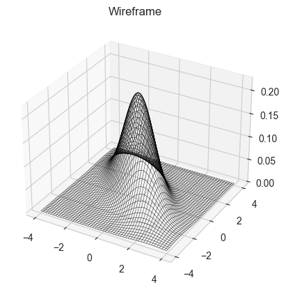
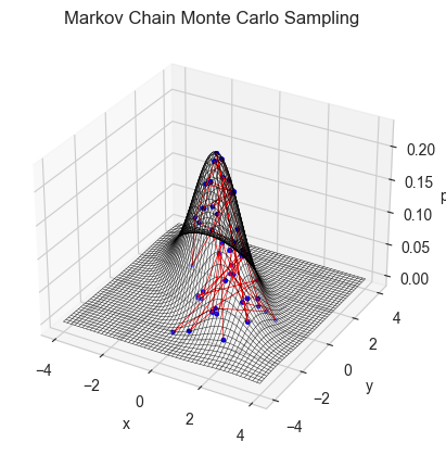
We will try to produce the samples for a multinormal Normal distribution:

# Code for MCMC sampling from a normal distribution
cov_matrix = jnp.array([[1,0.7],[0.7,1]])

def m_normal(x,y):
    mb_dist = cov_matrix[0,0]*(x**2) + (cov_matrix[0,1]+cov_matrix[1,0])*x*y + cov_matrix[1,1]*(y**2)
    return (1/(2*jnp.pi*jnp.sqrt(jnp.linalg.det(cov_matrix))))*jnp.exp(-0.5*(mb_dist))


x = jnp.linspace(-4,4,200)
y = jnp.linspace(-4,4,200)
X,Y = jnp.meshgrid(x,y)
Z = (vmap(m_normal))(X,Y)

fig = plt.figure()
ax = plt.axes(projection = '3d')
ax.plot_wireframe(X,Y,Z,color = 'black', lw = 0.3)
ax.set_title('Wireframe')

Text(0.5, 0.92, 'Wireframe')

print(random.uniform(random.PRNGKey(2), shape =(2,), maxval=1.0 , minval = -1.0) )
print(random.multivariate_normal(random.PRNGKey(1), mean =jnp.array([0.0,0.0]), cov = cov_matrix) )

[-0.703218    0.52689147]
[-0.11617039  1.4987264 ]

# Doing monte carlo optimisation on this function:-
x0 = 2.0; y0 = -3.0
n = 100

def small_unif_jump(key):
    return random.uniform(key, shape =(2,), maxval=0.4 , minval = -0.4)

def small_normal_jump(key):
    return random.multivariate_normal(key, mean =jnp.array([0.0,0.0]), cov = cov_matrix)

def monte_carlo_walk(fun, x0, y0, n, jump_f ,bounds = (np.array([-2,2]) ,np.array([-2,2])), ):
    xs = np.zeros(n); ys = np.zeros(n)
    keyval = 20
    xcurrent = x0; ycurrent = y0
    for i in range(n):
        keyval = keyval+1
        jump = jump_f(random.PRNGKey(keyval))
        x1 = xcurrent + jump[0]
        y1 = ycurrent + jump[1]
        # x1 = 0.2*random.normal(random.PRNGKey(i),shape = (1,)) + xcurrent
        # y1 = 0.2*random.normal(random.PRNGKey(i+1),shape = (1,)) + ycurrent
        if (x1 < bounds[0][0]) or (x1 > bounds[0][1]) or (y1 < bounds[1][0]) or (y1 > bounds[1][1]):
            x1 = xcurrent
            y1 = ycurrent
            i = i-1
            continue
        if fun(x1,y1) > fun(xcurrent,ycurrent):
            xcurrent = x1
            ycurrent = y1
        else:
            flip = random.uniform(random.PRNGKey(i+2),shape = (1,))
            if flip < fun(x1,y1)/fun(xcurrent,ycurrent):
                xcurrent = x1
                ycurrent = y1
            else:
                xcurrent = xcurrent
                ycurrent = ycurrent
        xs[i] = xcurrent; ys[i] = ycurrent
    return xs, ys

fig = plt.figure()
#xs, ys = monte_carlo_walk(m_normal, x0, y0, n, small_unif_jump, bounds = (np.array([-4,4]) ,np.array([-4,4])) )
xs, ys = monte_carlo_walk(m_normal, x0, y0, n, small_normal_jump, bounds = (np.array([-4,4]) ,np.array([-4,4])) )
ax = plt.axes(projection = '3d')
ax.plot_wireframe(X,Y,Z,color = 'black', lw = 0.3)
ax.scatter(xs,ys,m_normal(xs,ys),color = 'blue',s = 5)
ax.plot(xs,ys,m_normal(xs,ys),color = 'red',lw = 0.5)
ax.set_xlabel('x'); ax.set_ylabel('y'); ax.set_zlabel('pdf')
ax.set_title('Markov Chain Monte Carlo Sampling')

# Try to add slider, which actually works on jupyter book

Text(0.5, 0.92, 'Markov Chain Monte Carlo Sampling')

starting_points = [np.array([2.0,-3.0]),np.array([2.0,3.0]),np.array([-2.0,3.0]),np.array([-2.0,-3.0])]

fig, ax = plt.subplots(1, 4, figsize =(8, 2))
for sp in starting_points:
    n = 50
    xs, ys = monte_carlo_walk(m_normal, sp[0], sp[1], n, small_unif_jump, bounds = (np.array([-4,4]) ,np.array([-4,4])) )
    # ax[0].plot(xs,ys)
    ax[0].scatter(xs,ys,s = 5)
    # ax[0].set_xlabel('x'); ax[0].set_ylabel('y')
    ax[0].set_title('Uniform Jump')
    xs, ys = monte_carlo_walk(m_normal, sp[0], sp[1], n, small_normal_jump, bounds = (np.array([-4,4]) ,np.array([-4,4])) )
    # ax[1].plot(xs,ys)
    ax[1].scatter(xs,ys,s = 5)
    # ax[1].set_xlabel('x'); ax[1].set_ylabel('y')
    ax[1].set_title('Normal Jump')

n = 1000
x0 = 2.0; y0 = -3.0
xs, ys = monte_carlo_walk(m_normal, x0, y0, n, small_unif_jump, bounds = (np.array([-4,4]) ,np.array([-4,4])) )
ax[2].scatter(xs,ys,s = 5, lw = 0.5)
# ax[2].set_xlabel('x'); ax[0].set_ylabel('y')
ax[2].set_title('Uniform Jump')
xs, ys = monte_carlo_walk(m_normal, x0, y0, n, small_normal_jump, bounds = (np.array([-4,4]) ,np.array([-4,4])) )
ax[3].scatter(xs,ys,s = 5)
# ax[3].set_xlabel('x'); ax[1].set_ylabel('y')
ax[3].set_title('Normal Jump')

Text(0.5, 1.0, 'Normal Jump')

n = 10000
xs, ys = monte_carlo_walk(m_normal, x0,y0, n, small_unif_jump, bounds = (np.array([-4,4]) ,np.array([-4,4])) )

def plot3dhist(xs, ys, starts, ends, bins):
    z_hist = np.zeros((bins[0]+1, bins[1]+1))
    for i in range(len(xs)):
        z_hist[int((xs[i]-starts[0])/(ends[0]-starts[0])*bins[0])-1, int((ys[i]-starts[1])/(ends[1]-starts[1])*bins[1])-1] += 1

    x = jnp.linspace(starts[0],ends[0], bins[0]+1)
    y = jnp.linspace(starts[1],ends[1], bins[1]+1)
    X,Y = jnp.meshgrid(x,y)
    Z = z_hist/len(xs)
    fig = plt.figure()
    ax = plt.axes(projection = '3d')
    ax.plot_wireframe(X,Y,Z,color = 'black', lw = 0.3)
    ax.set_title('Wireframe')
    plt.show()

# plot3dhist(xs[5000:9999],ys[5000:9999],[-2,-2],[2,2],(50,50))
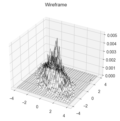
plot3dhist(xs,ys,[-4,-4],[4,4],(50,50))

3.1.5. Proof of Metropolis Algorithm

The metropolis algorithm seems to move around the complete domain space and produce samples in accordance with the pdf, but how do we proove that? The proof will be along the lines of the proof of stationarity of Markov chains, where we assumed that the probability vector \(p\) became equal to stationary distribution \(w\), and then we showed that afterwards, it stayed stationary to w as \(Pw = w\), (the Metropolis proof is on similar lines).

Proof

The proof that the sequence of iterations \( \theta_1, \theta_2, ...\) converges to the target distribution has two steps:

1. It is shown that the simulated sequence is a Markov chain with a unique stationary distribution

2. It is shown that the stationary distribution equals this target distribution.

The first step of the proof holds if the Markov chain is irreducible, aperiodic, and not transient. Except for trivial exceptions, the latter two conditions hold for a random walk on any proper distribution, and irreducibility holds as long as the random walk has a positive probability of eventually reaching any state from any other state; that is, the jumping distributions \(J_t\) must eventually be able to jump to all states with positive probability.

To see that the target distribution is the stationary distribution of the Markov chain generated by the Metropolis algorithm, consider that we have reached stationarity and are starting the algorithm at time \(t − 1\) with a draw \(\theta^{t−1}\) from the target distribution \(p(\theta|y)\).

Now consider any two such points \(\theta_a\) and \(\theta_b\), drawn from \(p(\theta|y)\) and labeled so that \(p(\theta_b|y) \ge p(\theta_a|y)\) . The unconditional probability density of a transition from \(\theta_a\) to \(\theta_b\) is

\[ p(\theta_{t-1} = \theta_a, \theta_{t} = \theta_b) = p(\theta_a|y)J_t(\theta_b|\theta_a) \]

where the acceptance probability is 1 because of our labeling of a and b, and the unconditional probability density of a transition from \(\theta_b\) to \(\theta_a\) is

\[ p(\theta_{t-1} = \theta_b, \theta_{t} = \theta_a) = p(\theta_b|y)Jt(\theta_a|\theta_b)(\frac{p(\theta_a|y)}{p(\theta_b|y)}) = p(\theta_a|y)J_t(\theta_b|\theta_a) \]

which is the same as the probability of a transition from \(\theta_a\) to \(\theta_b\), since we have required that \(J_t()\) be symmetric. Since the joint distribution of RVs \(\theta_{t-1}, \theta_{t}\) is symmetric, they have the same marginal distributions, and so \(p(\theta|y)\) is the stationary distribution of the Markov chain of \(\theta\).

Note we cannot be proove that it will necessarily reach stationarity, only that if does, then it remain constant after that. (Indeed, a lot of times MCMC sampling fails)