4.1. Graphical Models

Why graphical models

Graphical models are of fundamental importance to Probabilistic modeling as most relations and structures in models are represented in the form of graphical structures. They are also useful to demonstrate relations between random variables, parameters which comes handy when we have to make probabilistic programs to make inferences.

Definition

Graphical models refer to a family of probability distributions defined in terms of a directed or undirected graph.

Examples of Graphcial Models

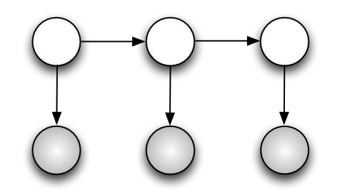
Note: All the circles in the graph are Random Variables. The shaded ones are observed variables (like \(y_i\)), variables that can be measured. The non shaded ones are latent variables, those that have to be infered (like \(\mu\)).

1. Markov Model

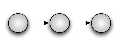
Fig. 4.1 Markov Model

2. Hidden Markov Model

Fig. 4.2 Hidden Markov Model

3. Mixture Model

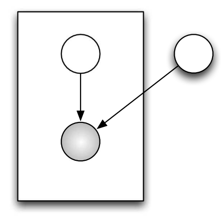
Fig. 4.3 Mixture Model

4.1.1. Directed Graphical Models

Directed Graphical Models are graphical model in which the edges have directions associated with them. Also known as Bayesian networks which are a useful representation for hierarchical Bayesian models. They form the foundation of applied Bayesian statistics (see e.g., the BUGS project). In such a model, the parameters are treated like any other random variable, and becomes nodes in the graph.

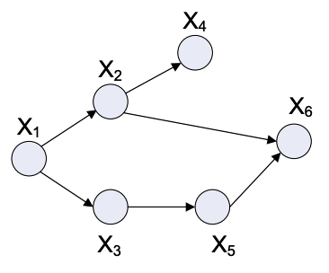
Fig. 4.4 Example Graph

Let \( {X_1, X_2, ... X_n } \) be a set of random variables, and \( {x_1, x_2, ... x_n } \) be a random sample.

Parents: We define \(\Pi_i\) as the set of parents of X_i. We will these definations to explore some important facts about these graphs.

For the example graph: \(\Pi_6 = {X_2, X_5}\) and \( \)

Topological Sort: A topological sort is a arrangement of random variables such that children come after parents. Ie all elements of set \(\Pi_i\), have index less than i.

For the example graph: \({1,2,3,4,5,6}\), and \({1,3,5,2,4,6}\)

Joint Probability: We can define the joint probability of the RV set as:

\[ p(x_{1:n}) = \prod_{i=1}^{n} p(x_i|x_{\pi_{i}}) \]

So for the example graph:

\[ p(x_{1:6}) = p(x_{1})p(x_{2}|x_1)p(x_3|x_1)p(x_4|x_2)p(x_5|x_3)p(x_6|x_2,x_5) \]

One of the main advantages of directed graph is that the joint distribution can be easily factored out based on the parents of nodes.

Causality: Directed Graphs are also popular as a path from A to B signifies a causal realtion between A and B.

4.1.1.1. Space Reduction

It is worth noting that epressing RV’s as graphs helps us reduce the space required. Consider the example with binary RV’s, as we have 6 RV’s it will require \(2^6 = 64\) data points to define distribution (joint). But notice that \(p(x_{1})\) takes only 2 values, \(p(x_{2}|x_1)\) takes 4 and \(p(x_6|x_2,x_5)\) takes 8 totalling, 26 for the joint distribution, hense saving space.

4.1.1.2. Conditional Independence

We want to understand when two or mulitple varaibles are independent of each other or independent conditional on value of some other variable being known. (Using I for independence symbol)

• Independence:

(4.1)\[\begin{align} X_A \; I \; X_B & \iff p(x_A, x_B) = p(x_A) p(x_B) \\ & \iff p(x_A | x_B) = p(x_A) \end{align}\]

• Conditional Independence:

(4.2)\[\begin{align} X_A \; I \; X_B | X_C & \iff p(x_A, x_B | x_C) = p(x_A|x_C) p(x_B|x_C) \\ & \iff p(x_A | x_B, x_C) = p(x_A|x_C) \end{align}\]

This means that if we know the value of \(X_C\), then the value of \(X_A\) does not depend on the value of \(X_B\). This is an important concept and comes in handy when we want to explore the dependencies of the features of the models.

In general, the conditional independence relationships encoded by a Bayes Net are best be explained by means of the “Bayes Ball” algorithm. At its core, it uses the below three fundamental examples to find independence.

4.1.1.3. Three Elementary Examples

1. Past-Present-Future Sequence

Fig. 4.5 Past-Present-Future Sequence

This graph represents the Markov chain where every Random Variable depends only on the one behind it.

Some properties:

Joint Distribution: \(p(x,y,z) = p(x)p(y|x)p(z|y)\)

Dependencies: \( X \; I \; Z | Y \), ie. value of X is independent of Z if we know the value of Y

2. Little Tree

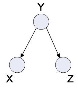
Fig. 4.6 Little Tree

Some Properties:

Joint Distribution: \(p(x,y,z) = p(y)p(x|y)p(z|y)\)

Dependencies: \( X \; I \; Z | Y \), just like the one above, here also Z is independent of X if Y is given otherwise, they may or may not be dependent.

3. Inverse Tree

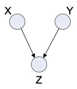
Fig. 4.7 Inverse Tree

The inverse tree is also a very elementary graph found in many models.

Properties:

Joint Distribution: \(p(x,y,z) = p(x)p(y)p(z|x,y)\)

Dependencies: Here we have a direct independence between \(X\) and \(Y\), but notably the conditional independence \( X \; I \; Z | Y \), as seen in the above ones are not true. Hense X and Y are independent if Z is not known, and dependent if Z is known.

4.1.2. Undirected Graphical Models

Undirected graphs are much harder to work with (especially when defining the joint probabilities) as there is no parent and child relation rather the dependence is mutual, (but they also are quite useful as more expressive). Also known as Markov random fields (MRV).

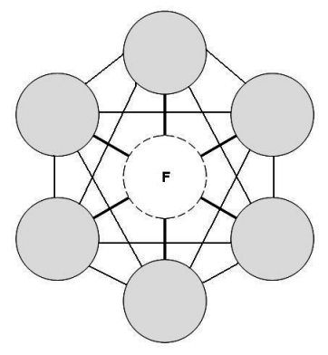
Fig. 4.8 Undirected Graph

4.1.2.1. Structure

1. Every node in an MRV, is conditionally independent of every other node in the network conditional on its direct neighbours. (Similar to directed graph)

2. We use potentials and graphs cliques to factorise the joint distribution (unlike the parent child factorisation)

3. We can give correlations between variables but no explicit way to generate samples (special case: gaussian processes)

4.1.2.2. Independence

While undirected graphs are more complicated than directed ones, independece finding is much more simpler.

Two (sets of) nodes A and B are conditionally independent given a third set, C, if all paths between the nodes in A and B are separated by a node in C.

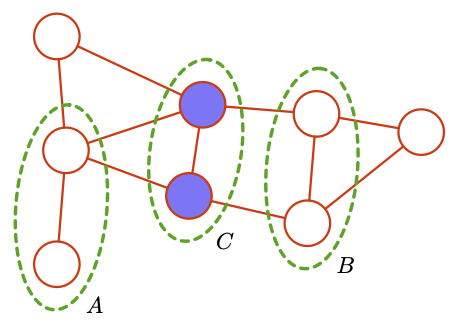
Fig. 4.9 Undirected Graph A,B,C

In this example we can see that the undirected graph has the \(A \; I\; B | C\), if there is even a single path between the two sets then independence will be broken.

We can use this info to get conditional independece, and construct factorised joint distribution.

4.1.2.3. Joint Probability

If we consider two nodes xi and xj that are not connected by a link, then these variables must be conditionally independent given all other nodes in the graph. This follows from the fact that there is no direct path between the two nodes, and all other paths pass through nodes that are observed, and hence those paths are blocked. This conditional independence property can be expressed as:

\[ p(x_i, x_j | x_{\backslash \{i,j\}}) = p(x_i | x_{\backslash \{i,j\}}) p(x_j | x_{\backslash \{i,j\}}) \]

This leads us to consider a graphical concept called a clique, which is defined as a subset of the nodes in a graph such that there exists a link between all pairs of nodes in the subset.

Hense, we can divide up the graph based on cliques and use potential functions (representative functions) to factorise the joint dist.

Let us denote a clique by C and the set of variables in that clique by \(x_C\) . Then the joint distribution is written as a product of potential functions \(\phi_C (x_C) \) over the maximal cliques of the graph

\[ p(x) = \frac{1}{Z} \prod_{C} phi_C (x_C) \]

Here the quantity Z, sometimes called the partition function, is a normalization constant and is given by (integrate if continous distribution):

\[ Z = \sum_{x} \prod_{C} phi_C (x_C) \]

4.1.2.4. Inference

The main challenge is to calculate the conditional probabilites and we will show the general method here.

Let f be the query node indexes, E be the evidence indexes, and R be the remaining indexes.

Goal: \( p(x_f | x_E) = \frac{p(x_f, x_E)}{p(x_E)} \)

1. Compute the marginal (integrate if continuous)

\[ p(x_f , x_E) = \sum_{x_R} p(x_f , x_E, x_R) \]

2. Compute the denominator (another marginal)

\[ p(x_E) = \sum_{x_f} p(x_f , x_E) \]

3. Take the ratio (goal)

\[ p(x_f | x_E) = \frac{\sum_{x_R} p(x_f , x_E, x_R)}{\sum_{x_f} p(x_f , x_E)} \]

4.1.3. Trees

Trees are important because many well known graphical models can be represented as trees, and some complicated ones can be approximated by trees. It is also the basis for the junction tree algorithm It is also the basis of an approximate inference algorithm.

4.1.4. Plates

Sometimes when describing graphical models, it is convenient to have a notation to indicate repeated structures. We use plates (or rectangular boxes) to enclose a repeated structure. We interpret this by copying the structure inside the plate N times, when N is indicated in the lower right corner of the plate.

Examples: A simple example would be a parametric gaussian model. Suppose we generate N i.i.d Samples from a gaussian distribution with mean \(\mu\), and standard deviation \(\sigma^2\)

\[ p(x_1, x_2, ... x_N, \mu, \sigma) = p(\mu)p(\sigma) \prod_{n = 1}^{N} p(x | \mu ,\sigma) \]

We can also represent it using plates as:-

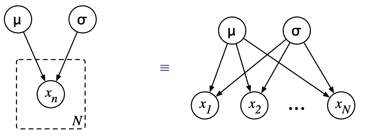
Fig. 4.10 Plates

https://www.cs.cmu.edu/~epxing/Class/10701-08s/Lecture/lecture18-GM1.pdf https://www.cs.ubc.ca/~murphyk/Bayes/bnintro.html https://mlg.eng.cam.ac.uk/zoubin/talks/lect2gm.pdf

4.1.5. Inferencing

Two lines on inferencing and use of these models.

4.1.6. Structure Learning

Two lines on structure learning

https://www.cs.ubc.ca/~murphyk/Papers/intro_gm.pdf

4.1.7. Examples

1. Factor Analysis and PCA

2. Kalman Filters, HMMs