5.3. Information Theory

In layman terms Data Analysis is the process of extracting useful information from data. But what is information? How do we measure it?

In this notebook, we will explore the concept of information, uncertainity in Random Variables and how it can be quantified. We will also be looking at a way to quantify the magnitude of an update from one set of beliefs to another using the concept of KL Divergence.

5.3.1. Entropy

Entropy is the average amount of “information”, “surprise”, or “uncertainty” inherent in the variable’s possible outcomes.

For a random variable $X$ with $n$ possible outcomes, the entropy $H(X)$ is defined as:

$$H(X)=-\sum _{i=1}^{n}p(x_i)\log p(x_i)$$

where $p(x_i)$ is the probability of the $i^{th}$ outcome.

Here we share a simple intution of entropy. Suppose we have two events x and y, then the info gained on observing both would be sum of info gained on observing x and y individually $h(x,y)=h(x)+h(y)$. Also, the probability will have the relation $p(x,y)=p(x)p(y)$. From this we can infer that $h(x)$ must be given by a logarithm of $p(x)$.

$$h(x)=-\log p(x)$$

Now, for a random variable $X$ with a state $x_1$, the info we gain on it occuring is $h(x_1)=-\log p(x_1)$, but it also only occurs with probability $p(x_1)$, so the average info we gain is $h(X)=-\sum _{i=1}^{n}p(x_i)\log p(x_i)$.

The base of the logarithm is arbitrary. If we use base 2, then the unit of information is the bit. If we use base e, then the unit of information is the nat. If we use base 10, then the unit of information is the digit.

Entropy as Length of Transmitted Code

If we have 8 states (a,b,c,d,e,f,g, h) with probabilities ($\frac{1}{2},\frac{1}{4},\frac{1}{8},\frac{1}{16},\frac{1}{64},\frac{1}{64},\frac{1}{64},\frac{1}{64}$) respectively, then the entropy is:

$$H(X)=-\frac{1}{2}\log \frac{1}{2}-\frac{1}{4}\log \frac{1}{4}-\frac{1}{8}\log \frac{1}{8}-\frac{1}{16}\log \frac{1}{16}-\frac{4}{64}\log \frac{1}{64}=-2$$

This means that on average, we need 2 bits to encode the state of the random variable. We can represent the codes as (a: 0, b: 10, c: 110, d: 1110, e: 111100, f: 111101, g: 111110, h: 111111). The pdf average length of the code is 2 bits.

Differential Entropy

The continuous version of entropy is called differential entropy. It is defined as:

$$H(X)=-{\int }_{-\mathrm{\infty }}^{\mathrm{\infty }}p(x)\log p(x)dx$$

Note, this can also be in negative as pdf can be greater than 1.

5.3.2. Joint Entropy

Joint entropy is the extension of entropy to multiple random variables. For two random variables $X$ and $Y$, the joint entropy $H(X,Y)$ is defined as:

$$H(X,Y)=-\sum _{i=1}^n\sum _{j=1}^{m}p(x_i,y_j)\log p(x_i,y_j)$$

where $p(x_i,y_j)$ is the joint probability of the $i^{th}$ outcome of $X$ and the $j^{th}$ outcome of $Y$.

5.3.3. Cross Entropy

Cross-entropy is a measure of the difference between two probability distributions for a given random variable or set of events. Note: on same set.

Till now, we have been looking at the entropy of a single random variable. But what if we have two random variables $X$ and $Y$ with the same set of outcomes? In this case, we can use the cross entropy to get a measure of the difference between the two probability distributions over the same underlying set of events.

$$H_{ce}=-\sum _{i=1}^{n}p(x_i)\log q(x_i)$$

The intution between why it gives a measure of the difference between the two probability distributions will become clearer after we look at KL Divergence.

It shows up in the Cross entropy loss function in logistic learning, where we are trying to minimize the difference between the actual output (a one hot vector, which acts like a probibility distribution), and the predicted distribution of probabilites for different classes.

5.3.4. Mutual Information

Mutual information is a measure of the amount of information that one random variable contains about another random variable.

For two random variables $X$ and $Y$, the mutual information $I(X;Y)$ is defined as:

$$I(X;Y)=\sum _{i=1}^n\sum _{j=1}^{m}p(x_i,y_j)\log \frac{p(x_i,y_j)}{p(x_i)p(y_j)}$$

It intuitively measures how much information is shared between the two random variables. If $X$ and $Y$ are independent, then $I(X;Y)=0$, and it increases the more dependent they become.

Here we can recognise that $\frac{p(x_i,y_j)}{p(x_i)p(y_j)}$, is the correlation between the two variables, and the mutual information is the expectation of the log of the correlation.

5.3.5. KL Divergence

KL Divergence is a measure of how one probability distribution is different from a second, reference probability distribution.

Information in itself is a vague and abstract concept. But we can quantify the magnitude of an update from one set of beliefs to another very well using the concept of KL Divergence. Here we will show the KL divergence formulae, understand some of its properties and relate them to entropy and cross entropy.

For two probability distributions $p(x)$ and $q(x)$, the KL divergence $D_{KL}(p||q)$ is defined as:

$$D_{KL}(p||q)=\sum _{i=1}^{n}p(x_i)\log \frac{p(x_i)}{q(x_i)}$$

In the continuous case, it is defined as:

$$D_{KL}(p||q)={\int }_{-\mathrm{\infty }}^{\mathrm{\infty }}p(x)\log \frac{p(x)}{q(x)}dx$$

This quantifies the information update on changing from prior belief $q(x)$ to posterior belief $p(x)$.

5.3.5.1. KLD properties

1. Continuity of KL Divergence

KL Divergence is continuous in the limit as $p\to 0$ and $q\to 0$.

The information gain should be continous. The KL divergence by its formulae is continous, but we have to check the cases where $p(x)=0$ and $q(x)=0$.

In the limit $p\to 0$, we have $\underset{p\to 0}{lim}p\log \frac{p}{q}\to 0$, so the KL divergence is continous at $p=0$.

For $q\to 0$, we have $\underset{q\to 0}{lim}p\log \frac{p}{q}\to \mathrm{\infty }$, but, this is expected as if $q$ (prior) is zero at some point, then if the posterior $p$ is non-zero at that point, then the information gain is infinite, as we had not expected the event to occur at all.

2. Non Negativity of KL Divergence

KL Divergence is non-negative, and is equal to zero if and only if $p(x)=q(x)$.

The information gain should be positive regardless of the probability distributions, as we always gain information on changing our beliefs.

We will make use of the Jensens Inequality, which states that for a convex function $f(x)$, we have:

$$f(\sum _i{\lambda }_i{x}_i)\le \sum _i{\lambda }_{i}f(x_i)$$

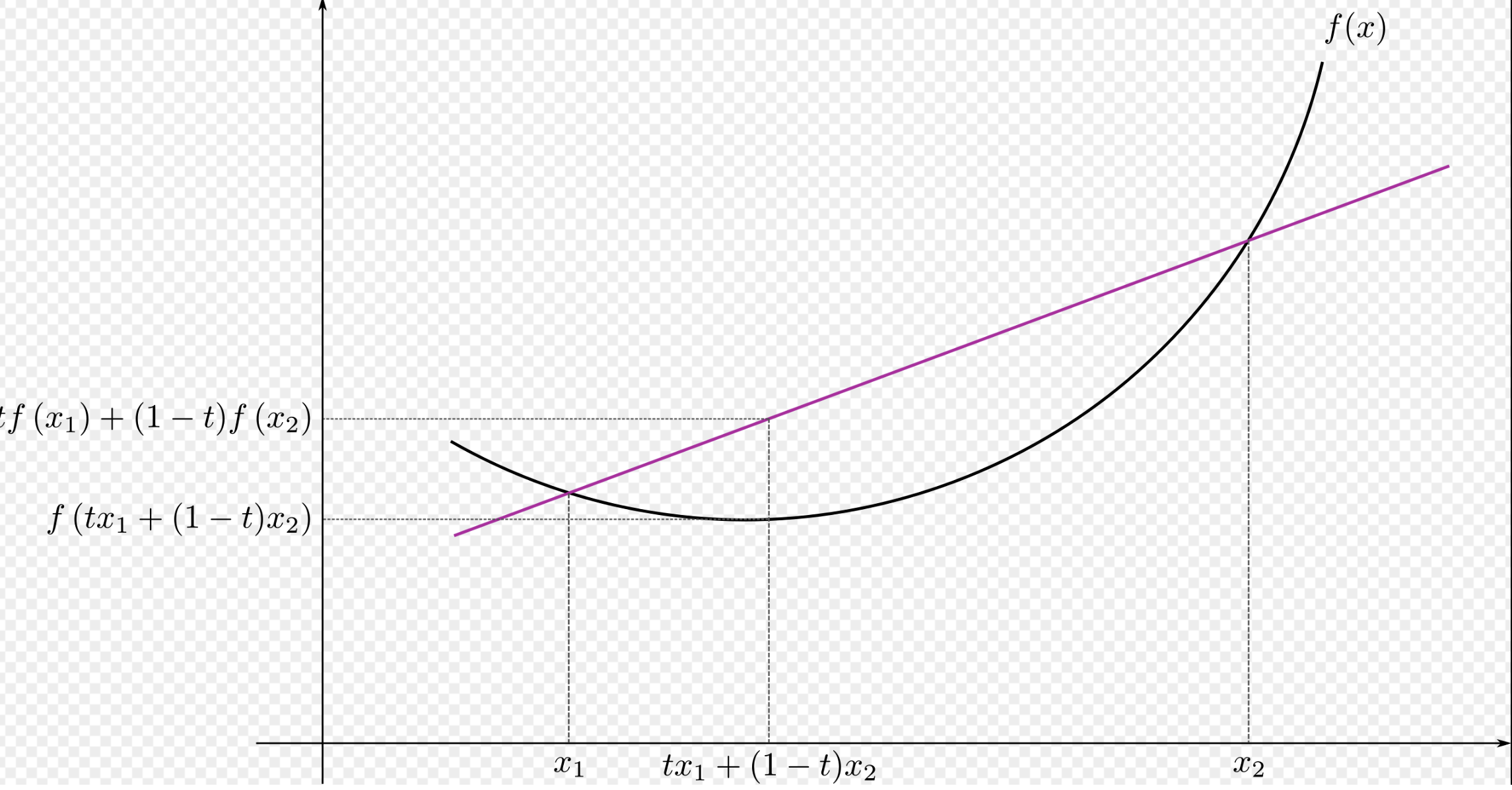
Fig. 5.1 Jensen Inequality

Jensens Inequality is the equation for the statement that in a convex function, all secant lines lie above the graph of the function. This is also evident by the figure above.

Proof: $D_{KL}(p||q)\ge 0$ with equality if and only if $p(x)=q(x)$

(5.7)$$\begin{array}{rl}-D_{KL}(p||q)& =-\sum _{x}p(x)\log \frac{p(x)}{q(x)}=\sum _{x}p(x)\log \frac{q(x)}{p(x)}\\ & \le \log \sum _{x}p(x)\frac{q(x)}{p(x)}=\log \sum _{x}q(x)=0\\ & \le \log \sum _{x}q(x)=log(1)=0\end{array}$$

The equality holds when $p(x)=q(x)$. Note: We used the fact that log is a concave function, so we can apply inverse Jensens Inequality.

The non-negativity of the KL divergence is a very important property, as it allows us to get bounds on expressions.

3. Chain Rule for KL Divergence

KL Diveregence is additive, i.e. $D_{KL}(p(x,y)||q(x,y))=D_{KL}(p(x)||q(x))+D_{KL}(p(y|x)||q(y|x))$

For probabilities we have the chain rule (product rule) as:

$$p(x,y)=p(x|y)p(y)=p(y|x)p(x)$$

Is there a similar rule for KL divergence? Can we split the information gain from two variables in a chain rule as we did for probabilities?

(5.8)$$\begin{array}{rl}{D}_{KL}(p(x,y)||q(x,y))& ={\int }_x{\int }_{y}dxdyp(x,y)\log \frac{p(x,y)}{q(x,y)}\\ & ={\int }_x{\int }_{y}dxdyp(x,y)[\log \frac{p(x)}{q(x)}+\log \frac{p(y|x)}{q(y|x)}]\\ & ={\int }_{x}dx\log \frac{p(x)}{q(x)}{\int }_{y}p(x,y)dy+{\int }_{x}p(x)dx{\int }_{y}p(y|x)\log \frac{p(y|x)}{q(y|x)}dy\\ & ={\int }_{x}dxp(x)\log \frac{p(x)}{q(x)}+{\int }_{x}p(x)D_{KL}(p(y|x)||q(y|x))dx\\ & =D_{KL}(p(x)||q(x))+D_{KL}(p(y|x)||q(y|x))\end{array}$$

Here we have put $D_{KL}(p(y|x)||q(y|x))$ inplace of ${\mathbb{E}}_{p(x)}[D_{KL}(p(y|x)||q(y|x))]$, as the expectation is taken over $p(x)$, and $p(y|x)$ is a function of $x$, so it is constant with respect to $p(x)$.

This means that just like the probabilities, we can also use a chain rule for the KL divergence. This is a very important property, as it allows us to split the information gain from multiple variables into individual information gains.

4. KL Divergence is invariant to reparametrisation

KL Divergence is invariant to reparametrisation of the variables.

What happens when we reparametrise our functions from $x\to y$, The KL Divergence should ideally not change, as we are just changing the way we are representing the same information, and it does not.

If we change the variable from $x\to y$, then we also have $p(x)dx=p(y)dy$

(5.9)$$\begin{array}{rl}{D}_{KL}(p(x)||q(x))& ={\int }_{x}p(x)\log \frac{p(x)}{q(x)}dx\\ & ={\int }_{y}p(y)\frac{dy}{dx}\log \frac{p(y)|\frac{dy}{dx}|}{q(y)|\frac{dy}{dx}|}dx\\ & ={\int }_{y}p(y)\log \frac{p(y)}{q(y)}dy\end{array}$$

Because of this reparameterization invariance we can rest assured that when we measure the KL divergence between two distributions we are measuring something about the distributions and not the way we choose to represent the space in which they are defined. We are therefore free to transform our data into a convenient basis of our choosing, such as a Fourier bases for images, without affecting the result.

5. KL Divergence is not Symmetric

KL Divergence is not symmetric, i.e. $D_{KL}(p(x)||q(x))\ne D_{KL}(q(x)||p(x))$

By looking at its formulae itself, we can say KL Divergence is not symmetric, but should’nt it be? After all the information gained on changing from $p(x)$ to $q(x)$ should be the same as the information gained on changing from $q(x)$ to $p(x)$. But, this seemingly obvious statement is not true. Case in point: The info gained on going from a neutral event to a rare event is lower than that of going from the rare event to the neutral event.

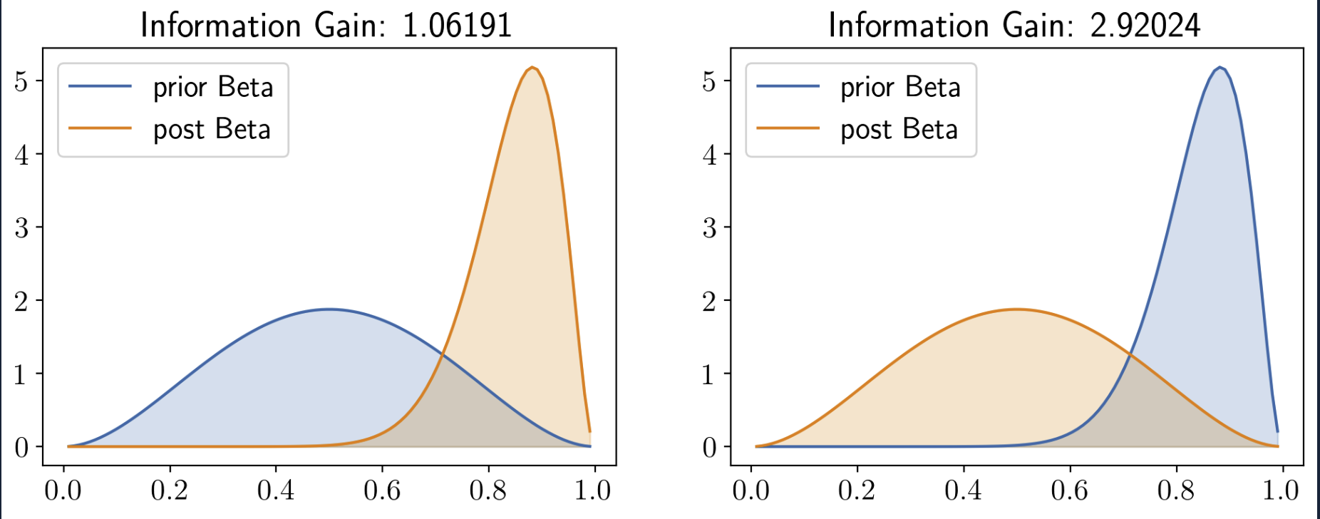
Fig. 5.2 Assymetry of KLD

In this example, we took two different Beta distributions, Beta1 = Beta($\alpha =3,\beta =3$) and Beta2 = Beta($\alpha =16,\beta =3$). This clearly shows our point. (Similar analysis can be done with the slider code given below)

As another Example:-

Suppose we have a biased coin: Initially we were told that it shows heads with a probability 0.443, and then told that no, actually it has a probability 0.975 of showing heads. The information gain is:

$$D_{KL}(p||q)=p{\log }_2\frac{p}{q}+(1-p){\log }_2\frac{1-p}{1-q}=1$$

If we flip the game then the information gained will be:-

$$D_{KL}(q||p)=q{\log }_2\frac{q}{p}+(1-q){\log }_2\frac{1-q}{1-p}=2$$

Thus we see that starting with a distribution that is nearly even and moving to one that is nearly certain takes about 1 bit of information, or one well designed yes/no question. To instead move us from near certainty in an outcome to something that is akin to the flip of a coin requires more persuasion.

import math
q = 0.443; p = 0.975
print("Info gain1: ", p*math.log2(p/q) + (1-p)*math.log2((1-p)/(1-q)))

p = 0.443; q = 0.975
print("Info gain2: ", p*math.log2(p/q) + (1-p)*math.log2((1-p)/(1-q)))

Info gain1:  0.9977011988907731
Info gain2:  1.9898899560575691

Calculating the beta distribution klds

import torch
import matplotlib.pyplot as plt
from ipywidgets import interact

def calc_info_gain(y1, y2):
    L = 200
    return 1/L*torch.sum(y2*torch.log(y2/y1))

def plot_beta(alpha1, beta1, alpha2, beta2):
    Beta1 = torch.distributions.Beta(concentration1=alpha1, concentration0=beta1)
    Beta2 = torch.distributions.Beta(concentration1=alpha2, concentration0=beta2)
    xs = torch.linspace(0.01, 0.99, 100)
    ys1 = Beta1.log_prob(xs).exp()
    plt.plot(xs, ys1, color='C0', label = "prior Beta")#label='Beta' + str(alpha1) + ',' + str(beta1))
    ys2 = Beta2.log_prob(xs).exp()
    plt.plot(xs, ys2, color='C1', label = "post Beta")#label = 'Beta' + str(alpha2) + ',' + str(beta2))
    plt.legend()
    # Filled area
    plt.fill_between(xs, ys1, color='C0', alpha=0.2)
    plt.fill_between(xs, ys2, color='C1', alpha=0.2)
    # write title with info gain only till 5 decimal places
    plt.title('Information Gain: ' + str(round(calc_info_gain(ys1, ys2).item(), 5)))

interact(plot_beta,alpha1=(1.0, 19, 1.0), beta1=(1.0, 19, 1.0), alpha2=(1.0, 19, 1.0), beta2=(1.0, 19, 1.0))

<function __main__.plot_beta(alpha1, beta1, alpha2, beta2)>

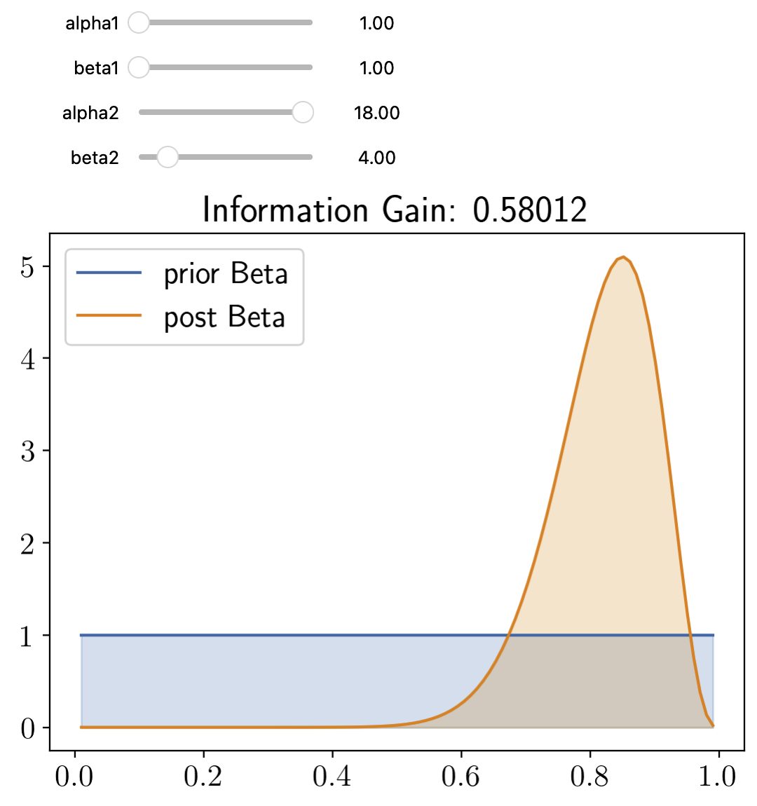
Fig. 5.3 Slider Example

5.3.5.2. Entropy and KLD

Entropy of a distribution p is a contant minus (-) the KL Divergence of that distribution from the uniform distribution.

The entropy of a distribution tries to capture the information, uncertainity of the pdf and the KL Divergence gives us the information gained on updating our belief of a pdf. So, it is natural to ask if there is a relation between the two.

For Discrete Case:

$$KLD=\sum _{i=1}^{n}p(x_i)\log \frac{p(x_i)}{q(x_i)},Entropy=-\sum _{i=1}^{n}p(x_i)\log p(x_i)$$

We can use $q_i=\frac{1}{n}$ as the uniform distribution, and we get:

(5.10)$$\begin{array}{rl}KLD& =\sum _{i=1}^{n}p(x_i)\log \frac{p(x_i)}{q(x_i)}\\ & =\sum _{i=1}^{n}p(x_i)\log \frac{p(x_i)}{\frac{1}{n}}\\ & =\sum _{i=1}^{n}p(x_i)\log p(x_i)+\sum _{i=1}^{n}p(x_i)\log n\\ & =\log n-Entropy\end{array}$$

Hense,

$$Entropy=constant-KLD$$

This also feels intuitive as the uniform distribution (U) is the most uncertain distribution, so it should have the maximum entropy and it does as it has the least KLD with U (ie 0).

It also makes sense in another way, as for any other distribution p, the more its KLD with U means more information gained on updating our belief from U to p, which means its prob is more peaked (certain), hense its lesser entropy, as shown by the formulae.

For Continuous Case:

Entropy is similar in the continuous case, where it is called continuous entropy, but with one change. Discrete entropy is always positive, but continuous entropy can be negative as pdf can be greater than 1. (Even U has Entropy 0, as log(1) = 0)

$$KLD={\int }_{}^{}p(x)\log \frac{p(x)}{q(x)}dx,Entropy=-{\int }_{}^{}p(x)\log p(x)dx$$

You can see from the slider example that the entropy of a distribution is a constant minus the KL Divergence of that distribution from the uniform distribution. (Set the prior as a beta dist of $\alpha =1,\beta =1$)

5.3.5.3. Cross Entropy and KLD

The cross entropy was our previous way to get some measure of closeness of two probability distributions and it is related to the KL Divergence.

(5.11)$$\begin{array}{rl}KLD& =\sum _{i=1}^{n}p(x_i)\log \frac{p(x_i)}{q(x_i)}\\ & =\sum _{i=1}^{n}p(x_i)\log p(x_i)-\sum _{i=1}^{n}p(x_i)\log q(x_i)\\ & =-H(p)+H_{ce}(p,q)\end{array}$$

Where $H_p$ is the entropy of the distribution $p$ and $H_{ce}$ is the cross entropy of the distributions $p$ and $q$.

$$H_{ce}(p,q)=-\sum _{i=1}^{n}p(x_i)\log q(x_i)$$

One way to think:-

In KLDivergence, we are trying to get the information gained on updating our belief from $q$ to $p$. Cross entropy gives us the uncertainity when we are trying to update our belief from $q$ to $p$ but using $q$ to encode the events. Entropy of $p$ gives us the uncertainity inherent in $p$. So on adding the KLDivergence and the entropy we get the cross entropy.

5.3.5.4. MI and KLD

MI measures the information gain if we update from a model that treats the two variables as independent p(x)p(y) to one that models their true joint density p(x, y).

KLDivergence and MI are obviously linked as KLD tells us how much info we gain on going from Y tp X, while MI gives us how much info of Y was being kept in X.

$$I(X;Y)=D_{KL}(p(x,y)||p(x)p(y))=\sum _{i=1}^n\sum _{j=1}^{m}p(x_i,y_j)\log \frac{p(x_i,y_j)}{p(x_i)p(y_j)}$$

Now, by formula, MI is measuring the information gained on updating our belief from $p(x)p(y)$ to $p(x,y)$. The divergence is zero if $p(x,y)=p(x)p(y)$, which means the two distributions are independent, which should give us a Mutual information 0 (which it does).

So the more $p(x,y)$ is different from $p(x)p(y)$, the more information they keep of each other, and the more MI they have.

Another interpretation:-

$$I(X;Y)=H(X)-H(X|Y)=H(Y)-H(Y|X)$$

So, MI is quantifies how uncertain we are about X - how uncertain we are about X given that we know Y, or it is the difference between the entropy of the random variable and the conditional entropy of the random variable given the other random variable. This means that MI is the information that the two random variables share with each other.

Thus we can interpret the MI between X and Y as the reduction in uncertainty about X after observing Y , or, by symmetry, the reduction in uncertainty about Y after observing X. Incidentally, this result gives an alternative proof that conditioning, on average, reduces entropy. In particular, we have $0\le I(X;Y)=H(X)-H(X|Y)$ ,and hence $H(X|Y)\le H(X)$.

We can also show that

$$I(X;Y)=H(X)+H(Y)-H(X,Y)$$

These relations are captured perfectly by this figure from Kevin Murphy

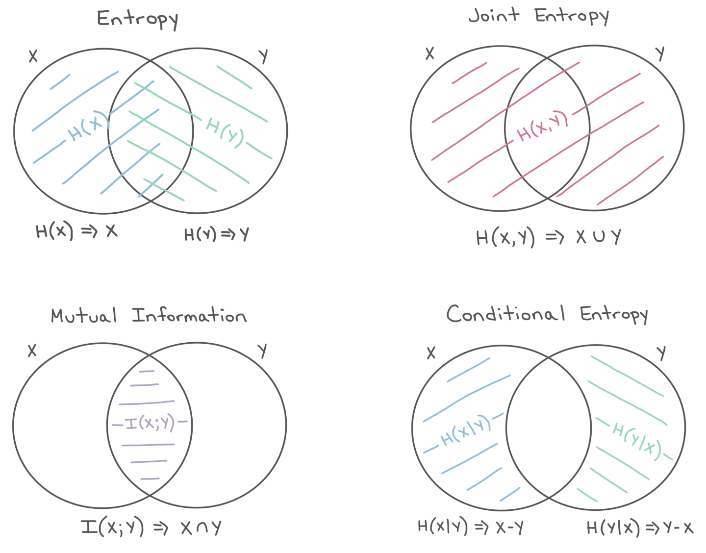
Fig. 5.4 Entropies

Information Of Data

How to charachterise the info of 111000 vs 100101 vs 101010?